Tuesday 29 December 2015

Locate Maximum Value-Reference & Lookup

Hello Exce-lent,

Happy holidays and how time flies....!

The past one month has been full of mixed feelings and reactions, from Sambogate to the recent Lagos drunk policeman, Stephen James who on Saturday 26th December, 2015 shot dead three male customers at a hotel in the Ketu area of Lagos State; Taiwo and Kehinde Oyesunle and their friend Jeje. A very unfortunate incident but I pray that the good Lord console their aged mother (75 years) and also protect and guide the rest of us as we move around preparing for the new year.

It has been a wonderful year, full of promises at the beginning, many fulfilled and many untouched as we read and most of these promises are now being carried over into the new year. Let me crave your indulgence to say that all hopes are not lost and in summary, permit me to also add that "He who is tired of learning, is tired of life"

I would like to wrap up our session for 2015 with this piece, which helps you locate the maximum data/ figure or information in a dataset. With KPIs being drawn at the end of the year to measure performances across board, a simple approach of a bank in showing appreciation to her customers might be to reward the highest deposit customer(s) for the year 2015. This sounds much of a possibility than rewarding the "highest withdrawal customer(s) for the year 2015, so let's walk down with this example.

Using FCMB for example, with branches nationwide and customers in different segments i.e Business Banking, Corporate Banking, HNI and all that, "my bank and I" can decide to reward the highest deposit customer for each of these segments. Simply put, a long list of customers running into hundreds of thousands (if not millions) would have to be queried or searched to have the highest customer with total deposit.

One can easily sort the list by Customer name and Amount (assuming we have a summed total of all transactions by customer) but a faster way to save some key strokes is using the "MAX" function in excel.


The MAX function above simple returns the maximum figure in the column. Please remember our assumption is that we are dealing with hundreds of thousands of customers and to quickly add this before you start doubting if excel can hold a banks full customer data, 2013 version of excel has over 16k + columns and about 1, 048, 567 rows per worksheet and there are 255 worksheet in a single workbook, uhm, now you believe! Adding INDEX/MATCH to this formula will also return the name of the customer as you may wish.

It could also be that the bank wants to reward more than one customer, (say the 5 highest) here the RANK function comes helpful. Whilst I developed an Excel Result computation sheet for my Alma mata, I used the MAX and RANK functions to identify the distinction student with the highest score and also ranked them accordingly. 

Join me from January 4th, 2016 as we discuss more on this but before then, I thank everyone who has made this year a success. To all my readers and co-learners, contributors and gurus, I say a big thank you and wish us all an Exce-lent 2016!

Remain Excel-lent!

Sorinola Oladapo
07014282477, 07062932708


Wednesday 25 November 2015

Extracting First Name, Middle names and Last names

Hello Excel-lent,

A friend recently asked if it was possible to extract first names, middle names and last names from a list of names and after thinking about it, I replied YES!

How is this done?

Let’s assume you have in;
  1.             Cell A1 the name “Sorinola Oladapo Augustine” 
  2.          And you want to extract the first name in cell B1, middle name in cell C1 and last name in cell D1 as shown in figure 1
  3.            In cell B1, type this formula =LEFT(A2,FIND(" ",A2)-1), without the double quotes as shown in       figure 2
  4.   In cell C1, type this formula =IF(LEN(B2&D2)+2>=LEN(A2),"",MID(A2,LEN(B2)+2,LEN(A2)-LEN(B2&D2)-2)) , without the double quotes as shown in figure 3
  5.    In cell D1, type this formula  =RIGHT(A2,LEN(A2)-FIND("*",SUBSTITUTE(A2," ","*",LEN(A2)-LEN(SUBSTITUTE(A2," ",""))))) , without the double quotes as shown in figure 4
  6.          If you have more than one name in column A, e.g A1: A10, copy cells B1: D1 and select cells B2:D10, then paste what you copied from B1:D1
  7.           Try is NOW and see, then share with others!


This has saved you a lot of time rather than having to retype the names one by one which off course is open to errors and typos. You don't have to cram the formula, they are text formulas that we have discussed about in the past. See links below;


Figure 1


Figure 2.


Figure 3


Figure 4


Excel-lently yours,

Sorinola Oladapo
07014282477, 07062932708
BB 52E9802D

Thursday 19 November 2015

Do you still have a Job?

Hello Excel-lent!

Good to be back here, hope your day has been good?

I got a BBM broadcast from a career "Pilot" yesterday and truthfully, it got me worried for some of us who are still in the rat race and since this platform is about being Excellent in all that you do, I felt I should share so that "as you aspire for the best, you're prepared for the worst". 

The lines below were from Jimi Tewe's broadcast of 11.18.2015, please read and digest!


"If you currently have a Job, you just might want to read this. 

This morning, I got a BBM broadcast from one of my contacts speaking about a Telecoms Company that recently let go of 30% of its workforce. 

Yesterday evening, I spent a few hours with a friend of mine who is very Senior in the Banking Industry and he confirmed the organised retrenchment efforts going on in the banking industry & the push to move back office staff to marketing functions.

The Oil & Gas industry is still reeling from the forced adjustment in staff numbers key players had to implement just to ensure business continuity. There will still be further cuts in the industry once inquisitions into subsidy fraud have been concluded by this anti-corruption driven government.

December is around the corner again. Typically, people get paid 3 times in some companies- Monthly Salary, 13th Month & Upfront payments.

I can confirm that HR Executives of some companies are also collating retrenchment & redeployment lists to help their business to cushion themselves against heavy payouts in this season.

As I am typing this, the sad reality is that someone you know might lose their job in a few weeks BUT in their thinking, they still have a Job.

The good news is that the economy is not only shrinking, it is changing and a few changes are birthing new opportunities. Only the discerning can know them.

Join me this evening on Twitter (follow @jimitewe) as I throw more light on Economic Realities, Organisational Responses and Personal Responsibility. 

The steering of your career lies in your hand.

It starts by 7.30pm and it WILL be explosive. Tell your friends, spouse, family members and colleagues about it. 

If you are not on Twitter... hmm.. I will talk about that also. 

Please rebroadcast. Many people think they still have a job. They just might be saved by your broadcast!

Jimi Tewe
Career Success Catalyst
Twitter: @jimitewe‎"

Of a truth, Economic Realities should not be disregarded on your path to Excellence. As a matter of fact, they dictate your survival in most instances but your ability to understand the realities of life, set your pace for growth. 

Do you still have a job?

Oladapo Sorinola
Business Intelligence & Data Analyst.

Thursday 15 October 2015

2.1. LOOKUP & REFERENCE - VLOOKUP PART 3

Hello Excel-lent,

In our last discussion on VLOOKUP,  we talked about VLOOKUP and its cousins HLOOUP, MATCH, INDEX and CHOOSE and also about many of us been used to One-column VLOOKUP. click here if you missed it please http://excelgist.blogspot.com.ng/2015/09/21-lookup-reference-vlookup-part-2.html

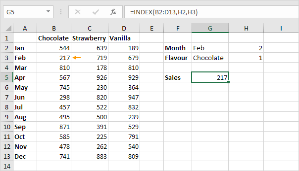
Now let's see how we can use VLOOKUP for a 2-way lookup in the below example. This example teaches you how to lookup a value in a two-dimensional range. We use the MATCH and INDEX function. Below you can find the sales of different ice cream flavors in each month.

1. To find the row number of Feb, use the MATCH function

Match Function

2. To find the column number of Chocolate, use the MATCH function.

Match Function

3. To find the sales of Chocolate in February, use the INDEX function.

Index Function

4. Put it all together.

Two-way Lookup Result

You can try replace the vanilla products using 3 Nigerian banks and see how it comes out, changing the months and the products or bank names as you wish to see the effect of the 2 column lookup.
We would not have achieved this using the VLOOKUP function alone, many thanks to it's cousins; MATCH & INDEX
Be good, be excel-lent!

Oladapo Sorinola
07014282477, 07062932708BB Pin 52E9802D


Wednesday 7 October 2015

Excel is 30!!! – what was your earliest memory of Excel?

Hello Excel-lent,

Last week Excel turned 30. As per wikipedia,
Microsoft released the first version of Excel for the Macintosh on September 30, 1985

Let's celebrate 30 years of Excel by reliving your first memory of it.

I will go first,
My first memory of Excel is from 2004. I just finished my accounting degree and assisted my department in building a simple automated "Result Manager" using Excel 2007.

The current result was manual and many student had suffered from its status as repeated carried over courses in lower levels where still reported as "FAILED" at final year even when students had retaken and "PASSED" those courses. I wanted to help and ensure students are not delayed or denied NYSC so i decided to automate the current result, starting from scratch. This was when I first used Excel, fully.


I made a spreadsheet with all the students details from Matric number to student names, courses and grades in details and worked on it all night. This was same year GLO started "mid night call promo" and most times when talking to my girlfriend at night for hours, while dozing off, I end up mumbling words like "CONCATENATE, VLOOKUP, IF, SUMIFS and bla bla bla...those words off-course got us "MATCHED". Her name is DUPE and I am DAPO. Collect like terms if you like.....

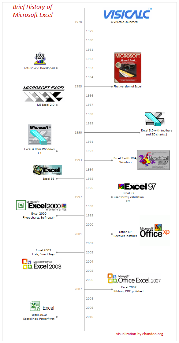
Here is a brief history of Microsoft Excel, in a visual time line

Brief History of Microsoft Excel - Timeline Visualization

Thanks to her (and many other things), I got paid for the little assistance and had since been "locked up" with Excel. I have designed payrolls and created Excel based reports and dashboards using VBA by fetching data from SQL databases and other data sources. This love for Excel made my life sweeter as an applications/ERP consultant. Today, I implement the 3rd largest global ERP application "INFOR SUNSYSTEMS"  and also provide deep training. 
What about you? What was your earliest memory of Excel? Please share in the comments or send a mail to me at sorinola@findataconsulting.com.
We are currently running a promo where you save at least NGN 2 Million from free implementation of Infor SunSystems as shown below. Take advantage!


Be Excel-lent.

Oladapo Sorinola
BB PIN 52E9802D
07014282477, 07062932708

Wednesday 30 September 2015

2.1. LOOKUP & REFERENCE - VLOOKUP PART 2

Hello Excel-lent,

Happy 55th Independence!

We started off with VLOOKUP during our last session but today, we will discuss about the VLOOKUP's COUSINS and they are HLOOUP, MATCH, INDEX and CHOOSE. I so much like these guys because they work as a team and always compliment each other.  VLOOKUP is restricted to leftmost columns but MATCH, INDEX and CHOOSE help VLOOKUP to search for data both ways....

VLookup

The VLOOKUP (Vertical lookup) function looks for a value in the leftmost column of a table, and then returns a value in the same row from another column you specify.
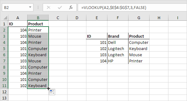
1. Insert the VLOOKUP function shown below.
VLookup Function in Excel

Explanation: the VLOOKUP function looks for the ID (104) in the leftmost column of the range $E$4:$G$7 and returns the value in the same row from the third column (third argument is set to 3). The fourth argument is set to FALSE to return an exact match or a #N/A error if not found.
2. Drag the VLOOKUP function in cell B2 down to cell B11.
Copy Vlookup Function
Note: when we drag the VLOOKUP function down, the absolute reference ($E$4:$G$7) stays the same, while the relative reference (A2) changes to A3, A4, A5, etc.

HLookup

In a similar way, you can use the HLOOKUP (Horizontal lookup) function.
HLookup Function

Match

The MATCH function returns the position of a value in a given range.
Match Function
Note: Yellow found at position 3 in the range E4:E7. The third argument is optional. Set this argument to 0 to return the position of the value that is exactly equal to lookup_value (A2) or a #N/A error if not found.

Index

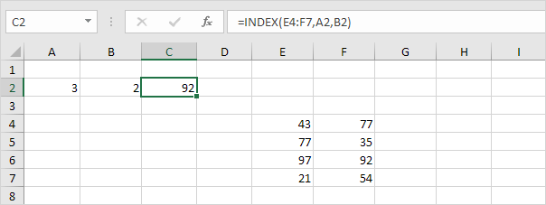
The INDEX function returns a specific value in a two-dimensional or one-dimensional range.
Index Function, Two-dimensional Range
Note: 92 found at the intersection of row 3 and column 2 in the range E4:F7.
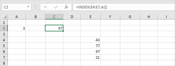
Index Function, One-dimensional Range
Note: 97 found at position 3 in the range E4:E7.

Choose

The CHOOSE function returns a value from a list of values, based on a position number.
Choose Function

Most people are familiar with One-column VLOOKUP but in our next class, we will discuss on how you can do a two-column VLOOKUP. Don't miss it!
Wishing you a happy 55th Independence celebration.
Excel-lently yours,
Oladapo Sorinola
07014282477, 07062932708
BB Pin 52E9802D

Tuesday 22 September 2015

2.1 Using Functions- LOOKUP & REFERENCE-VLOOKUP

Hello Excel-lent,

Let us start our session today with the VLOOKUP Function, basically because it is the most used of the lookup and Reference functions.

How the VLOOKUP Function Works
Excel's VLOOKUP function, which stands for "vertical lookup", can be used to look up specific information located in a table of data or database. VLOOKUP normally returns a single field of data as its output. How it does this is:

You provide a name or Lookup _value that tells VLOOKUP in which row or record of the data table to look for the desired information. You supply the column number - known as the Col_index_num - of the data you seek.

The function looks for the Lookup _value in the first column of the data table VLOOKUP then locates and returns the information you seek from another field of the same record using the supplied column number.

The VLOOKUP Function's Syntax and Arguments
A function's syntax refers to the layout of the function and includes the function's name, brackets, and arguments.

The syntax for the VLOOKUP function is:

= VLOOKUP (lookup_value, Table_array, Col_index_num, Range_lookup)

Lookup _value - (required) the value you want to find in the first column of the Table_array

Table_array - (required) this is the table of data that VLOOKUP searches to find the information you are after
- The Table_array must contain at least two columns of data
- The first column normally contains the lookup_value

Col_index_num - (required) the column number of the value you want found
- The numbering begins with the Lookup_value column as column 1
- If Col_index_num is set to a number greater than the number of columns selected in the range argument a #REF! error is returned by the function

Range_lookup - (optional) indicates whether or not the range is sorted in ascending order
- The data in the first column is used as the sort key
- A Boolean value - TRUE or FALSE are the only acceptable values
- If omitted, the value is set to TRUE by default
- If set to TRUE or omitted and an exact match for the Lookup _value is not found, the nearest match that is smaller in size or value is used as the search_key
- If set to TRUE or omitted and the first column of the range is not sorted in ascending order, an incorrect result might occur
- If set to FALSE, VLOOKUP only accepts an exact match for the Lookup _value

Let us discuss the diagram below. 


The table in the diagram above represents a company's employee database which shows employees Last Name, First Name, Department, Telephone Extension and Date Hired.

Given the Last Name only, you are required to find a staff's First Name, Department, Extension and Date Hired. Though Control + F button can help you locate one field at a time for less than 5 staffs conveniently but when you have a database of over 2,000 staffs, you are better off VLOOKUP.


Don't miss out on the sessions, Join Excelgist today to receive excel discussions straight in your mail box and do share this post with your colleagues.

Excel with Excel!

Excel-lently yours,
Oladapo Sorinola
07014282477, 07062932708
BB Pin 52E9802D

Monday 21 September 2015

2. Using Functions- LOOKUP & REFERENCE

Hello Excel-lent,

Today's traffic is what Prof. Wole Soyinka would call "mysterious millipede, moving towards a wailing wake-keep". Unfortunately, I cannot help you resolve these traffic issues within the metropolis but here I am to help you with the mostly used formulas in your everyday use of Microsoft Excel.

Someone recently asked in the Financial and Modelling group in Linkedin that " what function(s) of Excel do you use most?" and one word kept winning the day- VLOOKUP! 

In my years of excel experience as a data analyst, there is no way you can excuse yourself of the function "VLOOKUP" but you can garnish your data more and slice them deep and quicker with the introduction of other flavours like HLOOKUP, MATCH, INDEX, ROWS, COLUMNS, INDIRECT etc.

First, let us get to understand what each of these functions does.

ADDRESS      -    Returns a reference as text to a single cell in a worksheet
AREAS              -    Returns the number of areas in a reference
COLUMN      -    Returns the column number of a reference
COLUMNS      -    Returns the number of columns in a reference
HLOOKUP      -    Searches for a value in the top column of a table and then returns a value in the same                                     column from a row you specify in the table
HYPERLINK      -   Creates a shortcut that opens a document on your hard drive, a server, or the Internet
INDIRECT      -   Returns a reference indicated by a text value
MATCH              -   Returns the relative position of an item in an array
OFFSET              -   Returns a reference offset from a given reference
ROWS              -   Returns the number of rows in a reference
RTD                      -   Returns real-time data from a program that supports COM automation
GETPIVOTDATA -   Returns data stored in a PivotTable
CHOOSE       -   Chooses a value from a list of values
INDEX               -   Uses an index to choose a value from a reference or array
LOOKUP       -   Returns a value either from a one-row or one-column range or from an array
ROW               -   Returns the row number of a reference
TRANSPOSE      -    Returns the transpose of an array
VLOOKUP      -   Searches for a value in the leftmost column of a table and then returns a value in the                                       same row from a column you specify in the table

Interestingly, I use a combo of INDEX and MATCH to do the trick when I need to lookup towards the right which VLOOKUP cannot achieve.

Join me tomorrow as we begin to slice and dice your data with hundreds of Excel formulas and functions.

Join Excelgist today to receive excel discussions straight in your mail box and do share this post with your colleagues.

Excel with Excel!

Excel-lently yours,
Oladapo Sorinola
07014282477, 07062932708
BB Pin 52E9802D


Wednesday 9 September 2015

7 Best new features in Excel 2013.


Hello Awesome,

Today is a special day, it is the 9th day of September, 2015. Special because you and I are alive to witness it. All praise be to God. 
Whilst using the 2013 version of the Excel spreadsheet, I have come to appreciate the additional features that makes it more user friendly and time saving. A quick example is the Power View, Sparklines, Slicer and Timeline functions shown below. As a data analyst, they make my day all the time. 

 
Almost everyone will find something to appreciate in Excel 2013. It's more functional and easy to use. Everyone's going to love Flash Fill. Experienced number crunchers will appreciate the new data model feature. Inexperienced users forced to get more out of the application than their experience really supports will appreciate Recommended Charts, Recommended PivotTables, and Quick Analysis. The emphasis seems to be on easy access to features that were, prior to 2013, a bit harder to implement. These are the 7 new features that I think will benefits most users.

1. Flash Fill

Perhaps the closest thing to magic Excel users will ever see in a workbook is Flash Fill. This feature anticipates formatting and data requirements by recognizing patterns so it can finish what you start. Figure A shows a typical use for Flash Fill. First, I transposed a record's name value into last name, first name order. While doing the same for the second record, Flash Fill recognized a pattern and suggested possible entries to complete the column. When Flash Fill displays this list, you have two choices: Press Enter to complete the list or press [Esc] to remove it. 
Flash Fill can complete this list for you (Figure A): 


Excel_New_Ftrs.FigA.png

2. Recommended Charts

Most users don't always know the best chart type for their data. Recommended Charts takes the guesswork out of the process. Simply click inside the data you want to chart, click the Insert tab, and click Recommended Charts to see a collection of suggested chart types, as shown in Figure B. Then, click a thumbnail to preview your data as that chart type. Double-click a thumbnail to embed the chart. Using this feature lets you work with confidence knowing the chart will highlight your data in a meaningful way.


Excel_New_Ftrs.FigB.jpg

3: Recommended PivotTables

This feature works similar to Recommended Charts, but generates a quick PivotTable. It's a great new feature for most users, because so many of us struggle with PivotTables. Click inside the data range (which must have header cells) and click the Insert tab. In the Tables group, click Recommended PivotTables to display the dialog shown in Figure C. Select a thumbnail and click OK to embed an effective PivotTable in a new sheet.


Excel_New_Ftrs.FigC.jpg

PivotTables are a simple as a few clicks and a choice—no more struggling with field lists and table frames!

4: Quick Analysis

Use Quick Analysis to quickly preview your data in meaningful ways. For instance, Quick Analysis offers a second new way to generate appropriate charting for your data. Select the data and then click the Quick Analysis icon at the bottom-right, as shown in Figure D. Click the Charts tab to view the suggested chart types. If you don't see this icon, check your settings:
  1. Click the File tab and choose Options from the left pane.
  2. Choose General in the left pane (the default).
  3. In the User Interface Options section, the Show Quick Analysis Options On Selection option should be checked. Enabled is the default, so you should see this icon unless someone has changed this setting.
  4. Click OK.


Excel_New_Ftrs.FigD.jpg

Let Excel choose the most appropriate chart type!

5: Timelines

A timeline lets you filter records in a PivotTable—it works similar to a slicer, but you'll filter by dates. For instance, Figure E shows a PivotTable and timeline. (I used the same data range used in #3.) Once you have a PivotTable arranged, adding the timeline is simple:
  1. With the PivotTable selected, click the contextual Analyze tab.
  2. In the Filter group, click Insert Timeline.
  3. In the resulting dialog, check the date field (in this case, that's Date) and click OK. Excel will embed the timeline alongside the PivotTable.


Excel_New_Ftrs.FigE.jpg

Use the new Timeline with a PivotTable, it is just interesting!
To use the timeline, just drag the scroll bar or click a tile to further filter personnel totals by specific months. In the upper-right corner, you can change to years, quarters, months, and days. To clear the timeline filter, click the Clear button in the upper-right corner.

6: Data Model and Relationships

Excel 2013's new integrated data model support is well beyond a simple recommendation tip like this. You'll want to study and familiarize yourself with all of the possibilities:
  • Create PivotTables based on multiple tables.
  • Create one-to-one and one-to many relations between tables.
  • Easily connect to OData, Windows Azure DataMarket, and SharePoint.
  • Drill down to detail levels in a PivotTable or PivotChart.
  • Drill up for a high-end view.

7: New functions

Users often overlook new functions in a new version. This time around, you'll want to pay attention, as 2013 has several new functions that even casual users will want to know about. For a complete list, read New functions in Excel 2013. My favorite is DAYS(), which returns the number of days between two dates. The simple expression End Date – StartDate will return the same results, but having a short function is self-documenting, handier and simple.

Which 2013 excel feature(s) do you love most? Kindly share your experience using the comment space. 


To learn more about how excel can help you at your work place, join now to subscribe for daily excel tips or call me on 07014282477, 07062932708.


Sorinola Oladapo
BB Pin 52E9802D