Wednesday 30 September 2015

2.1. LOOKUP & REFERENCE - VLOOKUP PART 2

Hello Excel-lent,

Happy 55th Independence!

We started off with VLOOKUP during our last session but today, we will discuss about the VLOOKUP's COUSINS and they are HLOOUP, MATCH, INDEX and CHOOSE. I so much like these guys because they work as a team and always compliment each other.  VLOOKUP is restricted to leftmost columns but MATCH, INDEX and CHOOSE help VLOOKUP to search for data both ways....

VLookup

The VLOOKUP (Vertical lookup) function looks for a value in the leftmost column of a table, and then returns a value in the same row from another column you specify.
1. Insert the VLOOKUP function shown below.
VLookup Function in Excel

Explanation: the VLOOKUP function looks for the ID (104) in the leftmost column of the range $E$4:$G$7 and returns the value in the same row from the third column (third argument is set to 3). The fourth argument is set to FALSE to return an exact match or a #N/A error if not found.
2. Drag the VLOOKUP function in cell B2 down to cell B11.
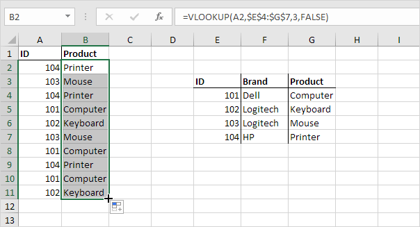
Copy Vlookup Function
Note: when we drag the VLOOKUP function down, the absolute reference ($E$4:$G$7) stays the same, while the relative reference (A2) changes to A3, A4, A5, etc.

HLookup

In a similar way, you can use the HLOOKUP (Horizontal lookup) function.
HLookup Function

Match

The MATCH function returns the position of a value in a given range.
Match Function
Note: Yellow found at position 3 in the range E4:E7. The third argument is optional. Set this argument to 0 to return the position of the value that is exactly equal to lookup_value (A2) or a #N/A error if not found.

Index

The INDEX function returns a specific value in a two-dimensional or one-dimensional range.
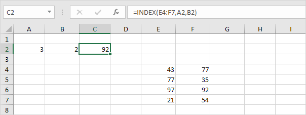
Index Function, Two-dimensional Range
Note: 92 found at the intersection of row 3 and column 2 in the range E4:F7.
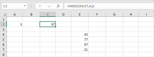
Index Function, One-dimensional Range
Note: 97 found at position 3 in the range E4:E7.

Choose

The CHOOSE function returns a value from a list of values, based on a position number.
Choose Function

Most people are familiar with One-column VLOOKUP but in our next class, we will discuss on how you can do a two-column VLOOKUP. Don't miss it!
Wishing you a happy 55th Independence celebration.
Excel-lently yours,
Oladapo Sorinola
07014282477, 07062932708
BB Pin 52E9802D

Tuesday 22 September 2015

2.1 Using Functions- LOOKUP & REFERENCE-VLOOKUP

Hello Excel-lent,

Let us start our session today with the VLOOKUP Function, basically because it is the most used of the lookup and Reference functions.

How the VLOOKUP Function Works
Excel's VLOOKUP function, which stands for "vertical lookup", can be used to look up specific information located in a table of data or database. VLOOKUP normally returns a single field of data as its output. How it does this is:

You provide a name or Lookup _value that tells VLOOKUP in which row or record of the data table to look for the desired information. You supply the column number - known as the Col_index_num - of the data you seek.

The function looks for the Lookup _value in the first column of the data table VLOOKUP then locates and returns the information you seek from another field of the same record using the supplied column number.

The VLOOKUP Function's Syntax and Arguments
A function's syntax refers to the layout of the function and includes the function's name, brackets, and arguments.

The syntax for the VLOOKUP function is:

= VLOOKUP (lookup_value, Table_array, Col_index_num, Range_lookup)

Lookup _value - (required) the value you want to find in the first column of the Table_array

Table_array - (required) this is the table of data that VLOOKUP searches to find the information you are after
- The Table_array must contain at least two columns of data
- The first column normally contains the lookup_value

Col_index_num - (required) the column number of the value you want found
- The numbering begins with the Lookup_value column as column 1
- If Col_index_num is set to a number greater than the number of columns selected in the range argument a #REF! error is returned by the function

Range_lookup - (optional) indicates whether or not the range is sorted in ascending order
- The data in the first column is used as the sort key
- A Boolean value - TRUE or FALSE are the only acceptable values
- If omitted, the value is set to TRUE by default
- If set to TRUE or omitted and an exact match for the Lookup _value is not found, the nearest match that is smaller in size or value is used as the search_key
- If set to TRUE or omitted and the first column of the range is not sorted in ascending order, an incorrect result might occur
- If set to FALSE, VLOOKUP only accepts an exact match for the Lookup _value

Let us discuss the diagram below. 


The table in the diagram above represents a company's employee database which shows employees Last Name, First Name, Department, Telephone Extension and Date Hired.

Given the Last Name only, you are required to find a staff's First Name, Department, Extension and Date Hired. Though Control + F button can help you locate one field at a time for less than 5 staffs conveniently but when you have a database of over 2,000 staffs, you are better off VLOOKUP.


Don't miss out on the sessions, Join Excelgist today to receive excel discussions straight in your mail box and do share this post with your colleagues.

Excel with Excel!

Excel-lently yours,
Oladapo Sorinola
07014282477, 07062932708
BB Pin 52E9802D

Monday 21 September 2015

2. Using Functions- LOOKUP & REFERENCE

Hello Excel-lent,

Today's traffic is what Prof. Wole Soyinka would call "mysterious millipede, moving towards a wailing wake-keep". Unfortunately, I cannot help you resolve these traffic issues within the metropolis but here I am to help you with the mostly used formulas in your everyday use of Microsoft Excel.

Someone recently asked in the Financial and Modelling group in Linkedin that " what function(s) of Excel do you use most?" and one word kept winning the day- VLOOKUP! 

In my years of excel experience as a data analyst, there is no way you can excuse yourself of the function "VLOOKUP" but you can garnish your data more and slice them deep and quicker with the introduction of other flavours like HLOOKUP, MATCH, INDEX, ROWS, COLUMNS, INDIRECT etc.

First, let us get to understand what each of these functions does.

ADDRESS      -    Returns a reference as text to a single cell in a worksheet
AREAS              -    Returns the number of areas in a reference
COLUMN      -    Returns the column number of a reference
COLUMNS      -    Returns the number of columns in a reference
HLOOKUP      -    Searches for a value in the top column of a table and then returns a value in the same                                     column from a row you specify in the table
HYPERLINK      -   Creates a shortcut that opens a document on your hard drive, a server, or the Internet
INDIRECT      -   Returns a reference indicated by a text value
MATCH              -   Returns the relative position of an item in an array
OFFSET              -   Returns a reference offset from a given reference
ROWS              -   Returns the number of rows in a reference
RTD                      -   Returns real-time data from a program that supports COM automation
GETPIVOTDATA -   Returns data stored in a PivotTable
CHOOSE       -   Chooses a value from a list of values
INDEX               -   Uses an index to choose a value from a reference or array
LOOKUP       -   Returns a value either from a one-row or one-column range or from an array
ROW               -   Returns the row number of a reference
TRANSPOSE      -    Returns the transpose of an array
VLOOKUP      -   Searches for a value in the leftmost column of a table and then returns a value in the                                       same row from a column you specify in the table

Interestingly, I use a combo of INDEX and MATCH to do the trick when I need to lookup towards the right which VLOOKUP cannot achieve.

Join me tomorrow as we begin to slice and dice your data with hundreds of Excel formulas and functions.

Join Excelgist today to receive excel discussions straight in your mail box and do share this post with your colleagues.

Excel with Excel!

Excel-lently yours,
Oladapo Sorinola
07014282477, 07062932708
BB Pin 52E9802D


Wednesday 9 September 2015

7 Best new features in Excel 2013.


Hello Awesome,

Today is a special day, it is the 9th day of September, 2015. Special because you and I are alive to witness it. All praise be to God. 
Whilst using the 2013 version of the Excel spreadsheet, I have come to appreciate the additional features that makes it more user friendly and time saving. A quick example is the Power View, Sparklines, Slicer and Timeline functions shown below. As a data analyst, they make my day all the time. 

 
Almost everyone will find something to appreciate in Excel 2013. It's more functional and easy to use. Everyone's going to love Flash Fill. Experienced number crunchers will appreciate the new data model feature. Inexperienced users forced to get more out of the application than their experience really supports will appreciate Recommended Charts, Recommended PivotTables, and Quick Analysis. The emphasis seems to be on easy access to features that were, prior to 2013, a bit harder to implement. These are the 7 new features that I think will benefits most users.

1. Flash Fill

Perhaps the closest thing to magic Excel users will ever see in a workbook is Flash Fill. This feature anticipates formatting and data requirements by recognizing patterns so it can finish what you start. Figure A shows a typical use for Flash Fill. First, I transposed a record's name value into last name, first name order. While doing the same for the second record, Flash Fill recognized a pattern and suggested possible entries to complete the column. When Flash Fill displays this list, you have two choices: Press Enter to complete the list or press [Esc] to remove it. 
Flash Fill can complete this list for you (Figure A): 


Excel_New_Ftrs.FigA.png

2. Recommended Charts

Most users don't always know the best chart type for their data. Recommended Charts takes the guesswork out of the process. Simply click inside the data you want to chart, click the Insert tab, and click Recommended Charts to see a collection of suggested chart types, as shown in Figure B. Then, click a thumbnail to preview your data as that chart type. Double-click a thumbnail to embed the chart. Using this feature lets you work with confidence knowing the chart will highlight your data in a meaningful way.


Excel_New_Ftrs.FigB.jpg

3: Recommended PivotTables

This feature works similar to Recommended Charts, but generates a quick PivotTable. It's a great new feature for most users, because so many of us struggle with PivotTables. Click inside the data range (which must have header cells) and click the Insert tab. In the Tables group, click Recommended PivotTables to display the dialog shown in Figure C. Select a thumbnail and click OK to embed an effective PivotTable in a new sheet.


Excel_New_Ftrs.FigC.jpg

PivotTables are a simple as a few clicks and a choice—no more struggling with field lists and table frames!

4: Quick Analysis

Use Quick Analysis to quickly preview your data in meaningful ways. For instance, Quick Analysis offers a second new way to generate appropriate charting for your data. Select the data and then click the Quick Analysis icon at the bottom-right, as shown in Figure D. Click the Charts tab to view the suggested chart types. If you don't see this icon, check your settings:
  1. Click the File tab and choose Options from the left pane.
  2. Choose General in the left pane (the default).
  3. In the User Interface Options section, the Show Quick Analysis Options On Selection option should be checked. Enabled is the default, so you should see this icon unless someone has changed this setting.
  4. Click OK.


Excel_New_Ftrs.FigD.jpg

Let Excel choose the most appropriate chart type!

5: Timelines

A timeline lets you filter records in a PivotTable—it works similar to a slicer, but you'll filter by dates. For instance, Figure E shows a PivotTable and timeline. (I used the same data range used in #3.) Once you have a PivotTable arranged, adding the timeline is simple:
  1. With the PivotTable selected, click the contextual Analyze tab.
  2. In the Filter group, click Insert Timeline.
  3. In the resulting dialog, check the date field (in this case, that's Date) and click OK. Excel will embed the timeline alongside the PivotTable.


Excel_New_Ftrs.FigE.jpg

Use the new Timeline with a PivotTable, it is just interesting!
To use the timeline, just drag the scroll bar or click a tile to further filter personnel totals by specific months. In the upper-right corner, you can change to years, quarters, months, and days. To clear the timeline filter, click the Clear button in the upper-right corner.

6: Data Model and Relationships

Excel 2013's new integrated data model support is well beyond a simple recommendation tip like this. You'll want to study and familiarize yourself with all of the possibilities:
  • Create PivotTables based on multiple tables.
  • Create one-to-one and one-to many relations between tables.
  • Easily connect to OData, Windows Azure DataMarket, and SharePoint.
  • Drill down to detail levels in a PivotTable or PivotChart.
  • Drill up for a high-end view.

7: New functions

Users often overlook new functions in a new version. This time around, you'll want to pay attention, as 2013 has several new functions that even casual users will want to know about. For a complete list, read New functions in Excel 2013. My favorite is DAYS(), which returns the number of days between two dates. The simple expression End Date – StartDate will return the same results, but having a short function is self-documenting, handier and simple.

Which 2013 excel feature(s) do you love most? Kindly share your experience using the comment space. 


To learn more about how excel can help you at your work place, join now to subscribe for daily excel tips or call me on 07014282477, 07062932708.


Sorinola Oladapo
BB Pin 52E9802D

Friday 4 September 2015

Quick weekend Poll

Hello Excel-lent,


Time for a quick weekend poll. What is your favorite tool for data analysis?


1. Formulas
2. Pivot Tables
3. Or both


Post your choice in the comments. Also mention the number of years Excel experience you have.


For ex, my answer is: Both (10 years)