Monday 31 August 2015

Your September Secret gift....

Hello Excel-lent,

I am glad to welcome you to September, how time flies!

I read Pastor Jimi Tewe's BB broadcast today on "DO IT BIG!" and he mentioned that "by this time tomorrow, we will have only 4 months left in 2015 and although you have done many things and accomplished a number of your goals, there is one thing you are yet to do..."

"When 2015 started, didn't you say to yourself that your accomplishment this year will be mind-blowing? So, apart from you, whose mind has been "blown?"

"Friend, it's time to do it BIG! If you are in Abuja next week Saturday (Sept 12) by 10am, join him as he holds his BIGGEST event in Abuja at (NAF Conference Centre) and it is absolutely free. To register, click this link;


What really touched me about his broadcast was when he asked "apart from you, whose mind has been blown?" I asked myself this same question over and over again and really wanted to know if I had in any way "blown" your mind through "Excelgist"?

I have no intent of "blowing" your mind, but at Excelgist blog, I have one goal, "to make you awesome in Excel and charting" but if you have your mind blown up in the process, then you're are simply excel-lent!

My secret gift for you this September is to learn how to un-protect a locked excel worksheet or workbook. I call it a secret gift because it opens up what's been hidden for you to see!

Do you have a protected Excel worksheet that you want to have full access to? Simply upload this worksheet to Google Spreadsheets using the url;


After uploading, open the worksheet and download it using the File menu and check through the locked cells and columns....I hope this revelation blows your mind!

Welcome to September!

Excel-lently yours,

Oladapo Sorinola
07014282477, 07062932708
BB Pin 52E9802D


Thursday 27 August 2015

1.5 -Working with the order of operations- "BODMAS"

Hello Excel-lent,

This topic brings back good old memories of our primary/elementary days in school when we were taught "Arithmetic" and a resounding "State and capital".... "Wow, things have changed!

Reciting through the "Times Table" was something I never liked then because of the long "Metric Arithmetical Tables"  that was more of a song....100 metre makes 1 kilometer, 365 days make 1 year, 366 days make 1 leap year and off course the long 2 times 1 two, 2 time 2 four, 2 time 3 six. I liked the State and capital more because of its rhythmic sequence, Sokoto- Sokoto, Ogun-Abeokuta, Niger-Minna, Plateau-Jos!....but today i am glad i did sang those songs using the book below in illustration 1. 

I almost forgot this- 30 days has September, April, June and November...

Illustration 1.


Picture source: http://www.nairaland.com/389532/u-did-not-use-exercise

Moving to higher classes, we were then exposed to one of the mathematical rules that turned on my hatred for "Quantitative Aptitude", why because I failed like no man's business and not until i learnt the simple rules behind BODMAS that i began to pass with good grades. 

BODMAS is the simple rule guiding the order of mathematical operations and the simple truth why you get some mathematical calculations wrong is because you flaw this rule. Now, let's go back to class as I still remember how the blackboard of St. Bernadette's Primary School, Abeokuta looks like

"Operations" mean things like add, subtract, multiply, divide, squaring, etc. If it isn't a number it is probably an operation.
But, when you see something like...
7 + (6 × 52 + 3)
... what part should you calculate first?

Start at the left and go to the right?
Or go from right to left?
Calculate them in the wrong order, and you will get a wrong answer !
So, long ago people agreed to follow rules when doing calculations, and they are:

Order of Operations

Do things in Brackets First. Example:
yes 6 × (5 + 3)=6 × 8=
48
 
no 6 × (5 + 3)=30 + 3=
33
(wrong)
Exponents (Powers, Roots) before Multiply, Divide, Add or Subtract. Example:
yes 5 × 22=5 × 4=
20
 
no 5 × 22=102=
100
(wrong)
Multiply or Divide before you Add or Subtract. Example:
yes 2 + 5 × 3=2 + 15=
17
 
no 2 + 5 × 3=7 × 3=
21
(wrong)
Otherwise just go left to right. Example:
yes 30 ÷ 5 × 3=6 × 3=
18
 
no 30 ÷ 5 × 3=30 ÷ 15=
2
(wrong)

How Do I Remember It All ... ? BODMAS !

 
B
Brackets first
O
Orders (ie Powers and Square Roots, etc.)
DM
Division and Multiplication (left-to-right)
AS
Addition and Subtraction (left-to-right)

The Order of Operations in Excel Formulas

Spreadsheet programs such as Excel and Google Spreadsheets have a number of arithmetic operators that are used in formulas to carry out basic mathematical operations such as addition and subtraction.

If more than one operator is used in a formula, there is a specific order of operations that Excel and Google Spreadsheets follow in calculating the formula's result

The Order of Operations is:

Brackets "( ) "
Orders (Powers and Square Roots, offs)
Division
Multiplication
Addition
Subtraction

An easy way to remember this is to use the acronym formed from the first letter of each word in the order of operations:

B O D M A S
How the Order of Operations Works

1. Any operation(s) contained in round brackets will be carried out first. 
2. Second, any calculations involving exponents will occur. 
3. After that, Excel considers division or multiplication operations to be of equal importance and carries out these operations in the order they occur left to right in the formula.
4. The same goes for the next two operations – addition and subtraction. They are considered equal in the order of operations. Whichever one appears first in an equation, either addition or subtraction is the operation carried out first.

Changing the Order of Operations in Excel Formulas
Since round brackets are first in the list, it is quite easy to change the order in which mathematical operations are carried out simply by adding brackets around those operations we want to occur first.

As simple as this may sound, using it wrongly has caused many companies to suffer financial loss arising from using bad Financial Models that does not obey the BODMAS rule. As a matter of fact, some employees salary has been wrongly calculated (shortchanged) from wrong use of BODMAS whilst calculating tax, prorated leave allowances and other deductions!

Some experience can be the worst teacher...


Excel-lently yours,

Oladapo Sorinola
07014282477, 07062932708
BB Pin 52E9802D

Monday 24 August 2015

1.4-Creating a basic formula -Part 2

Hello Excel-lent,

Welcome to the last week of August! A week full of expectations for both employer and employee, debtor and creditor.

Last week, we started out with creating a basic formula in excel and I recall mentioning that formulas are the engine room of Excel. We will continue this week, taking some deep look into how we can create basic formulas.

Creating a particular formula in excel, is determined by the issue at hand, that is, what mathematical, statistical or logical problem you want excel to solve for you? After identifying this problem and stating it then can you also identify the best formula to apply. There exists quite over 500 excel formula functions BUT you don't need to know them all, only learn and know the few ones that applies to your need and be able to reference them when you hear the call.

In Ms Excel, we have formulas ranging from Statistical to logical as shown in illustration 1 below and each of these formulas or a combo of them are helpful in solving operational issues.

Illustration 1.


Read http://excelgist.blogspot.com/2015/07/discover-these-15-extremely-powerful.html and http://excelgist.blogspot.com/2015/07/discover-these-15-extremely-powerful_6.html to see some TEXT & DATE functions and how they work.

For a creditor who had given out loans and wants to keep track of who is owing and repayments dates, a simple basic formula can be used on excel to track this just as we have in illustration 2 below.

Illustration 2.

As at today 24th of August, 2015, we are 65% and 235 days away into the year 2015, leaving out 129 days to go which represents 35%. How do we get this without marking or counting each day of the calendar? A simple "YEARFRAC" and "DAYS" formulas are used as shown below in illustration 3. If you decide to keep this simple calendar without updating the End Period date every day, you can simply type in "=TODAY()" formula where you have 8/24/2015 so that excel updates the date each time you open the worksheet.

Illustration 3.


Click " Join Excelgist " to receive Excelgist discussions directly to your mail box

Have a blessed week ahead.

Oladapo Sorinola
07014282477, 07062932708

Friday 21 August 2015

1.4-Creating a basic formula

Hello Excel-lent,

TGIF!

Hope you're doing great and how has your week been? The week has been tough emotionally but I thank God for His goodness and mercy! 

I was going to ask if you had ever used any excel formula before and for what purpose? That sounds like "are you serious at all?", but the factual truth is many have not seen the spreadsheet grid lines before or for those who had seen it, seeing was only what they could do!

We agreed last week that formulas are one of the most commonly used features of Excel and they can be used to carry out simple addition and subtraction or far more complex mathematical calculations. All formulas in Excel, no matter how complex, always begin with the same two steps:

  1.  Click on the cell where you want the formula's result to be displayed.
  2.  Type an equal sign ( = ) to let Excel know you are creating a formula
In the example below, I want my formula's result to be displayed in cell "B3", so i put my cursor in cell "B3" as shown below..

Illustration 1.

With that done, i can then think of what i want excel to calculate for me. I can do a basic calculation of how much i need to pay if i buy 25 litres of petrol at N87/ litre. In the example below, I have "Litres" entered in cell B1 and "Rate" in cell C1 as titles while i have 25 and 87 captured in cells B2 and C2 respectively. Because i want my formula's result to show in cell B3, i then type in the "equals to = sign" and using my cursor, reference cells B2 and C2 with a multiplication sign embedded like this =B2*C2. Once this is done, hit the enter button and gbam.....excel gives you your result.  

Illustration 2.

Illustration 3.
From this simple formula, you can then graduate to building complex formulas like what you see in Illustration 4 below.

Illustration 4.
With excel + a sound knowledge of formulas, you are bound to excel at your workplace and save a lot of time spent stumbling in a data jungle.

Please, if your answer is not 2,175 in the example above, kindly let me know but if you buy 25 litres Petrol at any filling station and they sell it for more than N2,175.00 (Two Thousand, One Hundred And Seventy Five Naira only) at N87 per litre, please report to DPR on 01-261 8228  or visit 5, Kofo Abayomi Street, Victorial Island, Lagos.

Have a Cntrl + A weekend, where "A" ="Awesome"

Oladapo Sorinola
07014282477, 07062932708
BB Pin 52E9802D


Thursday 13 August 2015

1.3- Entering and editing formulas

Hello Excel-lent,

I can't help you reduce Lagos traffic but i can help you work faster and be efficient at your workplace using Ms Excel. There is no reason why you shouldn't be excel-lent at work and that's the more reason why you should be part this and subsequent sessions of our Excel online training as we would be talking and discussing "FORMULAS".... the engine room of Excel J

In today's session, I would be introducing you to "how to enter and edit formulas" in Excel. There exists about over 500 formula in excel ranging from Statistical, Mathematics and Trigonometry,Financial, Engineering, Text, Date & Time, Lookup and Reference, Information, Database, Cube and Logical functions. You don't need to know them all but you need to be able to use the ones that speaks to your daily operational workplace need.

Excel Formula Overview


Formulas are one of the most commonly used features of Excel. They can be used to carry out simple addition and subtraction or far more complex mathematical calculations.

All formulas in Excel, no matter how complex, always begin with the same two steps:

  1.  Click on the cell where you want the formula's result to be displayed.
  2.  Type an equal sign ( = ) to let Excel know you are creating a formula.

Many formulas in Excel perform basic mathematical calculations such as subtraction and multiplication.

For these formulas, after the two steps listed above, we only need to add, in the correct order, the data to be used in the calculations and the mathematical operators that tell Excel which mathematical operation to perform.

Using Cell References in Formulas

Rather than enter the data directly into a formula, it is better to enter the cell references where the data is located into the formula.

The advantages of this are that:

  1.  If you later change your data the formula automatically updates to show the new result
  2.  In certain instances, using cell references makes it possible to copy formulas from one location to another in a worksheet

The easiest and best way to add cell references to a formula is to use pointing, which means to click with the mouse pointer on the cell containing the data you want added to the formula.

Click " Join Excelgist " to receive Excelgist discussions directly to your mail box.

Excel-lently yours,

Oladapo Sorinola
07014282477, 07062932708
BB Pin 52E9802D


Monday 10 August 2015

N500M legal suit for data error!

Hello Excellent,

On Tuesday, July 21st, 2015 when I shared "Eight of the worst spreadsheet blunders" http://excelgist.blogspot.com/2015/07/eight-of-worst-spreadsheet-blunders.html, it was very unfortunate that i couldn't lay my hands on any "local' sample as all the examples shared were foreign but what happened last week is an indication that "data error" has no boundary!

When an error occurs, it may take a whole lot of ones resources to clean out the mess, depending on the magnitude though but you will agree that a cleanser worth N500M  ($2.38M equivalent ) in law suit must have been a very BIG and MASSIVE error!


Image Source: Punch and ThisDay Newspapers, Friday 07, August 2015

Offcourse, the list must have been prepared by someone, and probably reviewed by another senior personnel but one thing people miss out on data is that Data is information and can either make or mar depending on how it's been processed. It could have been a case of errant cut-and-paste, it could have been this, it could have been that but my worry is that how did a name that is not meant to be on a Director's list appear on a Director's list? A Director of a company is not just an employee but someone who can be held liable for the operations or shortcomings of the company as in the case of  "Thriller Endeavours" and "Diamond Bank". This is a big data error and I wonder how many of this we have on banks databases. More shocking revelations may be revealed if we conduct a litmus test across board.

When University of Toledo lost $2.4M in Projected Revenue caused by "an internal budgeting error", President Daniel Johnson said "No job action would be taken against the employee who made the mistake, who has good performance record", I only wish same would be said and no job action would be taken against the employee or employees involved in this error.

Good a thing they have apologized, else N500M would have eaten down their profits for the year. You can read more here for full details
http://dailypost.ng/2015/08/07/diamond-bank-apologizes-to-abike-dabiri-for-erroneously-identifying-her-as-debtor/

http://leadership.ng/news/452279/debtors-list-abike-dabiri-slams-n500m-suit-on-diamond-bank

How excel-lent are you with Data? Judge yourself today before it is too late

Oladapo Sorinola
BB pin 52E9802D
07014282477, 07062932708


Tuesday 4 August 2015

1.2- Entering and editing text and values.

Hello Excel-lent,

Hope your week is turning out well. We started out last week on the basics with "Entering and Editing Data" and thank you for your calls and requests to subscribe by email. We have added the subscribe button for your convenience and you can now get the posts directly in your mail boxes once you key in your valid email address and click on the submit button. You will receive an activation notice that will welcome you to a new world of Excel-lent skills that will propel you at your workplace and transform you to an MVP- Most Valuable Player but one thing is, you only get better when you teach others! So let's share what we know, ask questions and make comments.....

The "Subscribe by email button" is located on the right hand side of the blog 


Now, back to work!
To enter text and values in an excel sheet, you need to first open up an excel sheet as shown below.


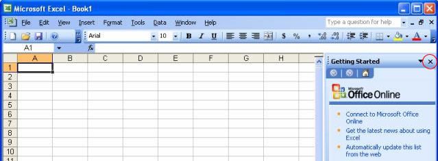
The screen shown here will appear.


The Title Bar
This lesson will familiarize you with the Microsoft Excel screen. You will start with the Title bar, which is located at the very top of the screen. On the Title bar, Microsoft Excel displays the name of the workbook you are currently using. At the top of your screen, you should see "Microsoft Excel - Book1" or a similar name. The position of "Book 1" depends on the version of Excel you are using.

The Menu Bar
The Menu bar is directly below the Title bar. The menu begins with the word File and continues with Edit, View, Insert, Format, Tools, Data, Window, and Help. You use a menu to give instructions to the software. Point with your mouse to a menu option and click the left mouse button. A drop-down menu opens. You can now use the left and right arrow keys on your keyboard to move left and right across the Menu bar. You can use the up and down arrow keys to move up and down the drop-down menu. To choose an option, highlight the item on the drop-down menu and press Enter. An ellipse after a menu item signifies additional options; if you choose that option, a dialog box opens.
Do the following exercise, which demonstrates using the Microsoft Excel menu bar.
  1. Point to the word File, which is located on the Menu bar.
  2. Click your left mouse button.
  3. Press the right arrow key until Help is highlighted.
  4. Press the left arrow key until Format is highlighted.
  5. Press the down arrow key until Style is highlighted. Press the up arrow key until Cells is highlighted.
  6. Press Enter to choose the Cells menu option.
  7. Point to Cancel and click the left mouse button to close the dialog box.
When using Microsoft Excel, you can set an option to tell Microsoft Excel to always show full menus or to show only the most frequently and recently used options. All the lessons in this tutorial assume you have your menus set to Always Show Full Menus. To set your menu to display full menus:
  1. Point to the word Tools, which is located on the menu bar.
  2. Click your left mouse button.
  3. Press the down arrow until customize is highlighted.
  4. Press Enter.
  5. Choose the Options Tab by clicking on it.
  6. If Always Show Full Menus does not have a check mark in it, click in the Always Show Full Menus box.
  7. Click Close to close the dialog box.
Toolbars
The Standard Toolbar


The Formatting Toolbar

Toolbars provide shortcuts to menu commands. Toolbars are generally located just below the Menu bar. Before proceeding with this lesson, make sure the toolbars you will use -- Standard and Formatting -- are available. Follow the steps outlined here:
  1. Point to View, which is located on the Menu bar.
  2. Click the left mouse button.
  3. Press the down arrow key until Toolbars is highlighted.
  4. Press the right arrow key.
  5. Both Standard and Formatting should have a check mark next to them. If both have a check mark next to them, press Esc two times to close the menu. If either does not have a check mark, press the down arrow key until Customize is highlighted.
  6. Press Enter. The Customize dialog box opens.
  7. Choose the Toolbars tab.
  8. Point to the box or boxes next to the unchecked word or words, Standard and/or Formatting, and click the left mouse button. A check mark should appear. Note: You turn the check mark on and off by clicking the left mouse button.
  9. Point to Close and click the left mouse button to close the dialog box.
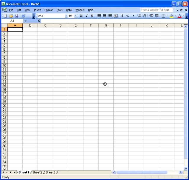
Worksheets
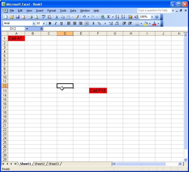
Microsoft Excel consists of worksheets. Each worksheet contains columns and rows. The columns are lettered A to IV; the rows are numbered 1 to 65536. The combination of a column coordinate and a row coordinate make up a cell address. For example, the cell located in the upper left corner of the worksheet is cell A1, meaning column A, row 1. Cell E10 is located under column E on row 10. You enter your data into the cells on the worksheet.
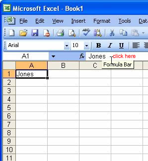
The Formula Bar
Formula Bar

If the Formula bar is turned on, the cell address displays in the Name box on the left side of the Formula bar. Cell entries display on the right side of the Formula bar. Before proceeding, make sure the Formula bar is turned on.
  1. Point to View, which is located on the Menu bar.
  2. Click the left mouse button. A drop-down menu opens. On the drop-down menu, if Formula Bar has a check mark next to it, the Formula bar is turned on. Press the Esc key to close the drop-down menu.
  3. If Formula Bar does not have a check mark next to it, press the down arrow key until Formula Bar is highlighted; then press Enter. The Formula bar should now appear below the toolbars.
  4. Note that the current cell address displays on the left side of the Formula bar.
The Status Bar
 
Status Bar

If the Status bar is turned on, it appears at the very bottom of the screen. Before proceeding, make sure the Status bar is turned on.
  1. Point to View, which is located on the Menu bar.
  2. Click the left mouse button. A drop-down menu opens.
  3. On the drop-down menu, if Status Bar has a check mark next to it, it is turned on. Press the Esc key to close the drop-down menu.
  4. If Status Bar does not have a check mark next to it, press the down arrow key until Status Bar is highlighted; then press Enter. The Status bar should now appear at the bottom of the screen.
Notice the word "Ready" on the Status bar at the lower left side of the screen. The word "Ready" tells you that Excel is in the Ready mode and awaiting your next command. Other indicators appear on the Status bar in the lower right corner of the screen. Here are some examples:
The Num Lock key is a toggle key. Pressing it turns the numeric keypad on and off. You can use the numeric keypad to enter numbers as if you were using a calculator. The letters "NUM" on the Status bar in the lower right corner of the screen indicate that the numeric keypad is on.
  • Press the Num Lock key several times and note how the indicator located on the Status bar changes.
The Caps Lock key is also a toggle key. Pressing it turns the caps function on and off. When the caps function is on, your entry appears in capital letters.
  • Press the Cap Lock key several times and note how the indicator located on the Status bar changes.
Other functions that appear on the Status bar are Scroll Lock and End. Scroll Lock and End are also toggle keys. Pressing the key toggles the function between on and off. Scroll Lock causes the movement keys to move the window without moving the cell pointer. End lets you jump around the screen. We will discuss both of these later in more detail.
Make sure the Scroll Lock and End indicators are off and complete the following exercises.
The Down Arrow Key
You can use the down arrow key to move downward one cell at a time.
  1. Press the down arrow key several times.
  2. Note that the cursor moves downward one cell at a time.
The Up Arrow Key
You can use the Up Arrow key to move upward one cell at a time.
  1. Press the up arrow key several times.
  2. Note that the cursor moves upward one cell at a time.
The Tab Key
You can use the Tab key to move across the page to the right, one cell at a time.
  1. Move to cell A1.
  2. Press the Tab key several times.
  3. Note that the cursor moves to the right one cell at a time.
The Shift+Tab Keys
You can hold down the Shift key and then press the Tab key to move to the left, one cell at a time.
  1. Hold down the Shift-key and then press Tab.
  2. Note that the cursor moves to the left one cell at a time.
The Right and Left Arrow Keys
You can use the right and left arrow keys to move right or left one cell at a time.
  1. Press the right arrow key several times.
  2. Note that the cursor moves to the right.
  3. Press the left arrow key several times.
  4. Note that the cursor moves to the left.
Page Up and Page Down
The Page Up and Page Down keys move the cursor up and down one page at a time.
  1. Press the Page Down key.
  2. Note that the cursor moves down one page.
  3. Press the Page Up key.
  4. Note that the cursor moves up one page.
The End Key
The End key, used in conjunction with the arrow keys, causes the cursor to move to the far end of the spreadsheet in the direction of the arrow.
  1. Press the End key.
  2. Note that "END" appears on the Status bar in the lower right corner of the screen.
  3. Press the right arrow key.
  4. Note that the cursor moves to the farthest right area of the screen.
  5. Press the END key again.
  6. Press the down arrow key. Note that the cursor moves to the bottom of the screen.
  7. Press the End key again.
  8. Press the left arrow key. Note that the cursor moves to the farthest left area of the screen.
  9. Press the End key again.
  10. Press the up arrow key. Note that the cursor moves to the top of the screen.
Note: If you have entered data into the worksheet, the End key moves you to the end of the data area.
The Home Key
The Home key, used in conjunction with the End key, moves you to cell A1 -- or to the beginning of the data area if you have entered data.
  1. Move the cursor to column J.
  2. Stay in column J and move the cursor to row 20.
  3. Press the End key.
  4. Press Home.
  5. You should now be in cell A1.
Moving Quickly Around the Worksheet
The following are shortcuts for moving quickly from one cell to a cell in a different part of the worksheet.
Go to -- F5
The F5 function key is the "Go To" key. If you press the F5 key while in the Ready mode, you are prompted for the cell to which you wish to go. Enter the cell address, and the cursor jumps to that cell.
  1. Press F5. The Go To dialog box opens.
  2. Type J3.
  3. Press Enter. The cursor should move to cell J3.
Go to -- Ctrl-G
You can also use Ctrl-G to go to a specific cell.
  1. Hold down the Ctrl key while you press "g" (Ctrl-g). The Go To dialog box opens.
  2. Type C4.
  3. Press Enter. You should now be in cell C4.
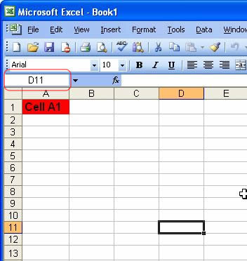
Name Box
You can also use the Name box to go to a specific cell.
  1. Type D11 in the Name box
  2. Press Enter. You should now be in cell D10.
Scroll Lock
Scroll Lock moves the window, but not the cell pointer.
  1. Press the Page Down key.
  2. Press Scroll Lock. Note "SCRL" appears on the Status bar in the lower right corner of the screen.
  3. Press the up arrow key several times. Note that the cursor stays in the same position and the window moves upward.
  4. Press the down arrow key several times. Note that the cursor stays in the same position and the window moves downward.
  5. Press Scroll Lock to turn the Scroll Lock function off.
  6. Hold down the Ctrl key and press Home to move to cell A1.
Selecting Cells
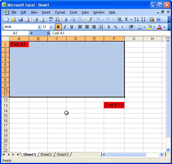
If you wish to perform a function on a group of cells, you must first select those cells by highlighting them. To highlight cells A1 to E1:
  1. Place the cursor in cell A1.
  2. Press the F8 key. This anchors the cursor.
  3. Note that "EXT" appears on the Status bar in the lower right corner of the screen. You are in the Extend mode.
  4. Click in cell E7. Cells A1 to E7 should now be highlighted.
  5. Press Esc and click anywhere on the worksheet to clear the highlighting.
Alternative Method: Selecting Cells by Dragging
You can also highlight an area by holding down the left mouse button and dragging the mouse over the area. In addition, you can select noncontiguous areas of the worksheet by doing the following:
  1. Place the cursor in cell A1.
  2. Hold down the Ctrl key. Do not release it until you are told. Holding down the Ctrl key enables you to select noncontiguous areas of the worksheet.
  3. Press the left mouse button.
  4. While holding down the left mouse button, use the mouse to move from cell A1 to E7.
  5. Continue to hold down the Ctrl key, but release the left mouse button.
  6. Using the mouse, place the cursor in cell G8.
  7. Press the left mouse button.
  8. While holding down the left mouse button, move to cell I17. Release the left mouse button.
  9. Release the Ctrl key. Cells A1 to E7 and cells G8 to I17 are highlighted.
  10. Press Esc and click anywhere on the worksheet to remove the highlighting.
Entering Data
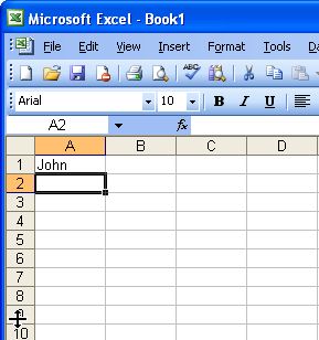
In this lesson, you are going to learn how to enter data into your worksheet. First, you place the cursor in the cell in which you would like to enter data. Then you type the data and press Enter.
  1. Place the cursor in cell A1.
  2. Type John Adeola.
  3. The Backspace key erases one character at a time. Erase "Adeola" by pressing the backspace key until Adeola is erased.
  4. Press Enter. The name "John" should appear in cell A1.
Editing a Cell
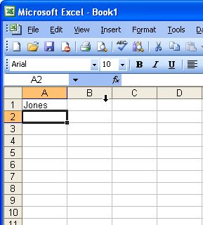
After you enter data into a cell, you can edit it by pressing F2 while you are in the cell you wish to edit.
  1. Move the cursor to cell A1.
  2. Press F2.
  3. Change "John" to "Jones."
  4. Use the backspace key to delete the "n" and the "h."
  5. Type nes.
  6. Press Enter.
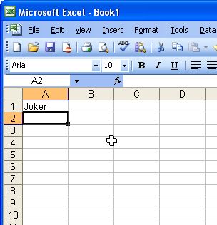
Alternate Method: Editing a Cell by Using the Formula Bar
You can also edit the cell by using the Formula bar. You can change "Jones" to "Joker" as follows:
  1. Move the cursor to cell A1.
  2. Click in the formula area of the Formula bar.
  1. Use the backspace key to erase the "s," "e," and "n."
  2. Type ker.
  3. Press Enter.
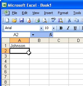
Alternate Method: Editing a Cell by Double-Clicking in the Cell
You can change "Joker" to "Johnson" as follows:
  1. Move the cursor to cell A1.
  2. Double-click in cell A1.
  3. Press the End key. Your cursor is now at the end of your text.
  4. Use the backspace to erase "r," "e," and "k."
  5. Type hnson.
  6. Press Enter.
Changing a Cell Entry
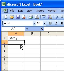
Typing in a cell while you are in the Ready mode replaces the old cell entry with the new information you type.
  1. Move the cursor to cell A1.
  2. Type Cathy.
  3. Press Enter. The name "Cathy" should replace "Johnson."
Wrapping Text
When you enter text that is too long to fit in a cell into a cell, it overlaps the next cell. If you do not want it to overlap the next cell you can wrap the text.
  1. Move to cell A2.
  2. Type Text too long to fit.
  3. Press Enter.
  4. Return to cell A2.
  5. Choose Format > Cells  from the menu.
  6. Choose the Alignment tab.
  7. Click Wrap Text.
  8. Click OK. The text wraps.
Deleting a Cell Entry
To delete an entry in a cell or a group of cells, you place the cursor in the cell or highlight the group of cells and press Delete.
  1. Place the cursor in cell A2.
  2. Press the Delete key.
Entering Numbers as Labels or Values
In Microsoft Excel, you can enter numbers as labels or as values. Labels are alphabetic, alphanumeric, or numeric text on which you do not perform mathematical calculations. Values are numeric text on which you perform mathematical calculations. If you have a numeric entry, such as an employee number, on which you do not perform mathematical calculations, enter it as a label by typing a single quotation mark first.
Enter a number:
  1. Move the cursor to cell B1.
  2. Type 200.
  3. Press Enter.
The number 200 appears in cell B1 as a numeric value. You can perform mathematical calculations using this cell entry. Note that by default the number is right-aligned.
Enter a value:
  1. Move the cursor to cell C1.
  2. Type '200.
  3. Press Enter.
The number 200 appears in cell C1 as a label. Note that by default the cell entry is left-aligned and a green triangle appears in the upper left corner of the cell.
Smart Tags
When you make an entry that Microsoft Excel believes you may want to change, a smart tag appears. Smart tags give you the opportunity to make changes easily. Cells with smart tag in them appear with a green triangle in the upper left corner. When you place your cursor in the cell, the Trace Error icon appears. Click on the Trace Error icon and options appear. When you made your entry in cell C1 in the previous section, a smart tag should have appeared.
  1. Move to cell C1.
  2. Click on the Trace Error icon. An options list appears. You can convert the label to a number, obtain help, ignore the error etc.
Saving a File
This is the end of Lesson1.2. To save your file:
  1. Choose File > Save  from the menu.
  2. Go to the directory in which you want to save your file.
  3. Type lesson1.2 in the File Name field.
  4. Click on Save. Alternatively, you can press the shortcut key combination of "ctrl" + S.

Closing Microsoft Excel
Close Microsoft Excel.
  1. Choose File > Close  from the menu.
Thank you for your time and do have an excel-lent week ahead.

Oladapo Sorinola
07062932708, 07014282477